Oufti Application

Segmentation

Segmentation can now be performed in an interactive window without the need to memorize the different segmentation parameters. There are three algorithms that are used for segmentation (Laplacian of Gaussian, valley, and cross detection) and they can be chosen by activating the radio button right next to them.

1.

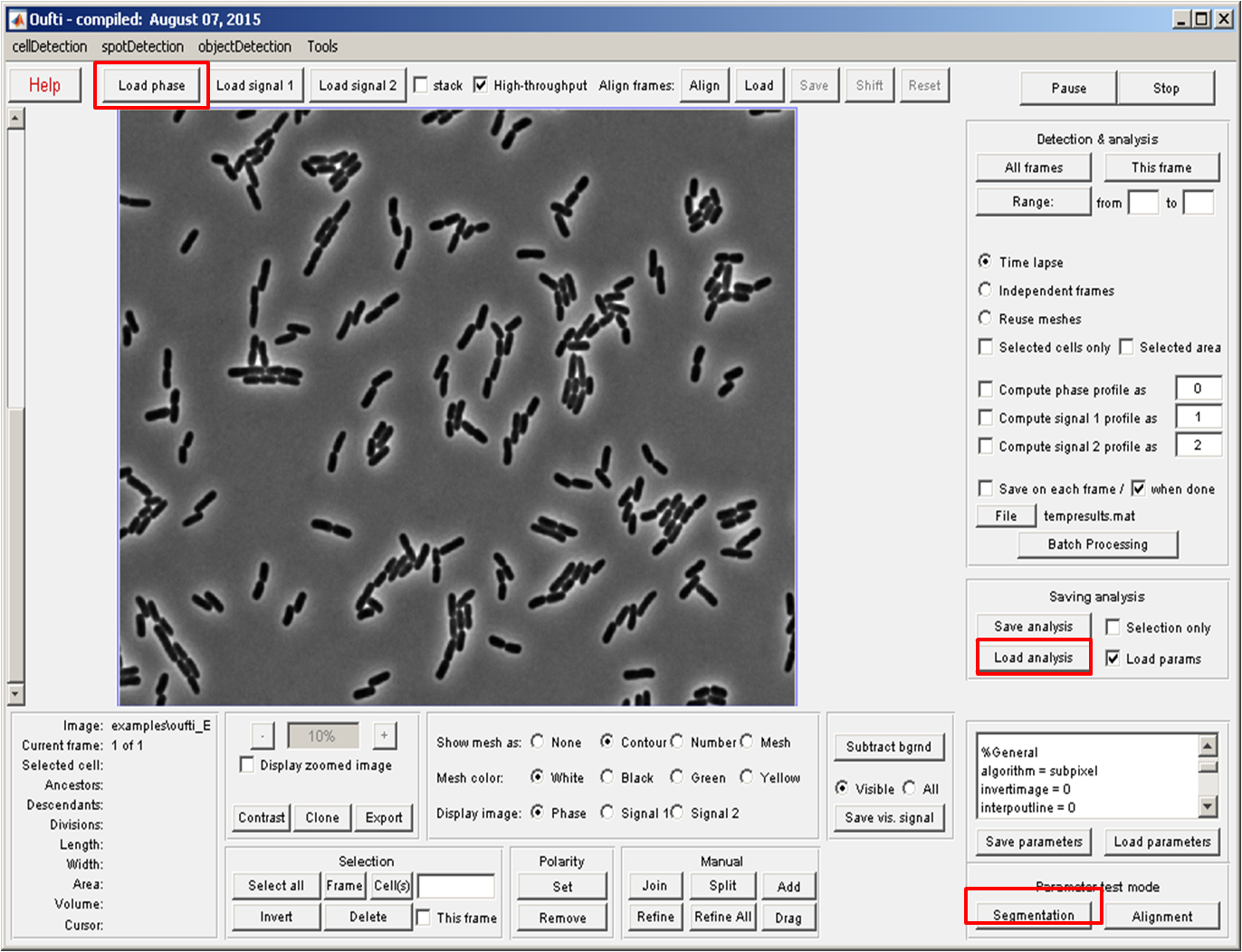
Launch Oufti window and then load the phase images by clicking Load phase button. Once images are loaded, click on File button to choose a location where final analysis will be saved.

2.

Click the Segmentation button in the lower right corner to perform segmentation.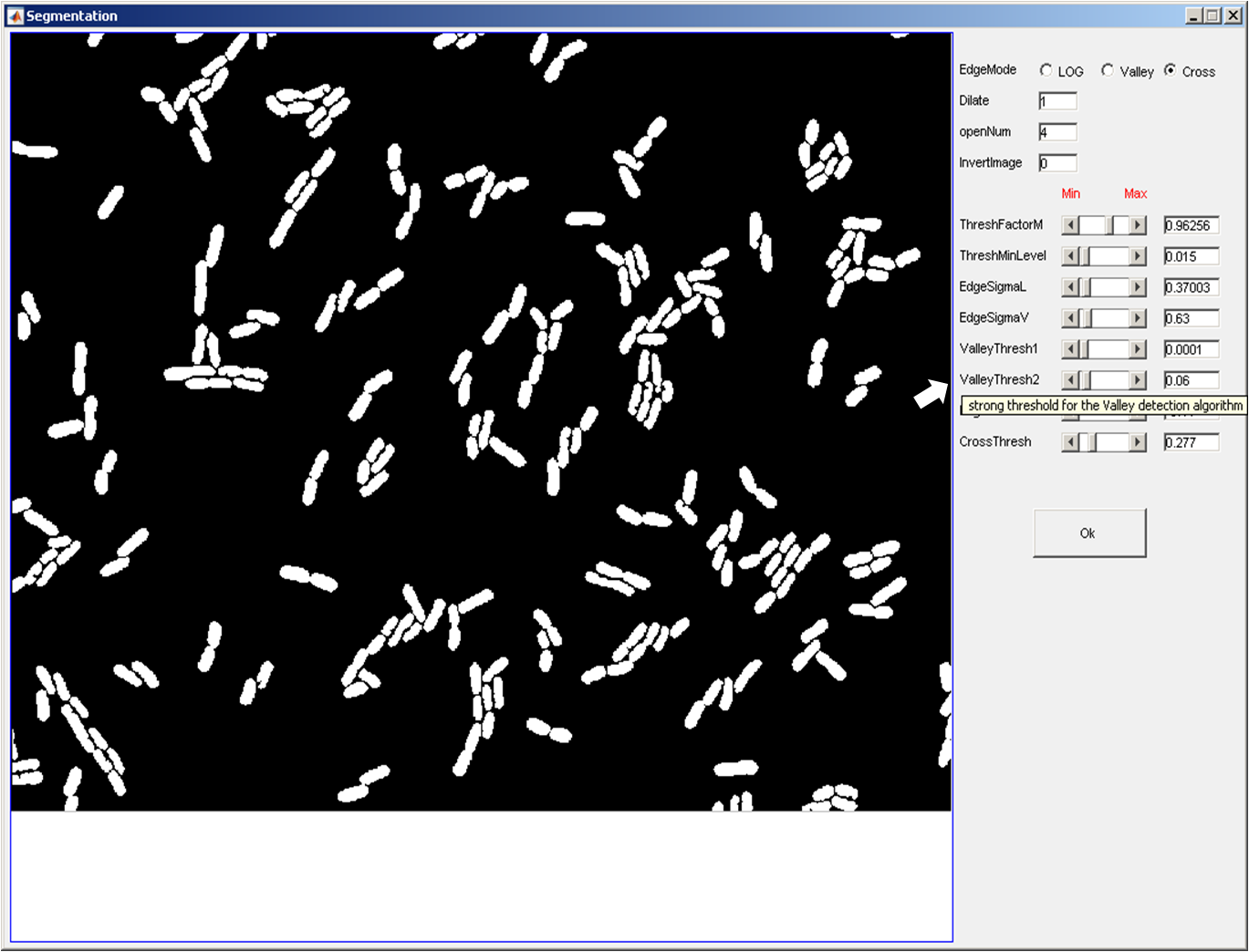

3.

Since the parameter file downloaded with mesh file contained segmentation paramters, there is no need to update paramters. However, one can hover a mouse on top of the parameter names to find its meaning and relevant application. Notice the interactive nature of the segmentation module, subtle changes in the highlighted parameters will change the segmentation result accordingly.

Note that the different algorithm selection correspond to activation and deactivation of various parameters. This makes it easy to interact with only those parameters that belong to a particular algorithm. If the OK button is not pressed before the window is closed, segmentation parameters will not be saved and the segmentation will not change.

cellDetection

Cell detection can be done using two algorithms -- pixel and subpixel. Subpixel detection is slower but more precise than pixel based algorithm. To see a quick tutorial on how cell detection is done go here

The Oufti Tools tab offers post-processing modules that one can use to view cell statistics and analysis plots. Click here for more information.

Adjusting parameters

This section details how to adjust and choose parameters to generate the best results for your data set. For a detailed description of what each parameter represents see the Parameters page. Once you have selected parameters that result in good cell outlines, save the parameter set. Saved parameter sets can be loaded and re-used for future data sets. Old parameter sets can be retrieved for use in new data sets, from either an old cellList file (open the .mat file, and the parameters used for that cellList file will appear) or a text file (.set).

1. Algorithm

For filamentous rod-shaped bacteria subpixel algorithm is used.
Use subpixel algorithm when detecting cell outlines throughout a time-lapse, and when cells are closely packed.
Pixel algorithm works well with irregular shaped cells.
Pixel algorithm is the fastest as it does not use the active contour step at all. This algorithm has poorer performance in separating cells in clusters and in tracking them in timelapses.
If you are using pixel algorithm, consider using it with (getmesh=1) or without (getmesh=0) meshes. Generation of meshes takes additional time, but may fail for irregularly-shaped cells. A mesh is required to produce a coordinate system inside, but frequently only the outline of the cell is sufficient.

3. Other shape-related parameters

Area. The program rejects the cells larger and smaller than a certain thresholds, which are regulated by the areaMin and areaMax parameters and expressed in pixels. To get an estimation of areaMin and areaMax, manually add a cell outline by clicking on Add button in Manual operation panel. Next, add points from end-to-end to the largest and the smallest cell in a given frame. To get an area in pixels for the two cells, click on each one and the area will be shown in the lower left panel of the GUI.
Smoothing cell. The program uses Fourier smoothing keeping a predefined number of descriptors, defined by fsmooth parameter. Typically for extremely small cells fsmooth should be ~ 10, for normal-size cells ~20, for filamentous cells up to ~200. Values too small don't allow to fit a complex shape of a cell correctly. Values too large are more tolerable, but may result in a pixilated outline.
Cell diameter (algorithm subpixel only) is controlled by parameters listed below;
- cellwidth sets the absolute value for the cell width. Note that this is not exact; for each individual cell the width will be adjusted to fit the outline.
- meshWidth sets a determined value for the initial mesh generation. This acts a starting point for fitting and producing initial cell outlines.
- wspringconst determines the rigidity of these parameters. Increasing the value of this parameter puts greater restriction on the determination of each cell’s width, and your resultant values will stay very close to the set cellwidth (default is ~0.5). For datasets in which you want greater flexibility, and a higher tolerance to alterations from the set cellwidth decrease this parameter. Decreasing this value to ~0.05 will produce mesh widths that are not strongly restricted to the set cellwidth and will allow the value to be solely determined from the cell outline.
Cell rigidity (algorithm subpixel only, for filamentous cells). The rigidity of filamentous cells is regulated by rigidityB (elasticity between nodes, < 10, default: 4) and rigidityRangeB (number of affected nodes, < cell length, default: 7) parameters. Low values make the cell too 'flexible', producing kinks sometimes resulting in errors. High values smooth kinks too much, so that the program may lose the cell.

4. Aligning the shape

Attraction/repulsion. Attraction is pulling the cell outline into the 'dark' (i.e. cell) areas to fill the cell completely. Repulsion is retracting the outline from 'light' (background) areas so that it does not extend from the cell. These effects help to fit better isolated cells, but may cause the shape to penetrate into the neighbor cell. The two effects are regulated by attrCoeff and repCoeff parameters. Typical values: from 0 to 1. Usually set them in the range 0-0.2 and adjust only if necessary. In most cases keep attrCoeff < repCoeff.
Alignment testing tool. The 'alignment' button on the 'Parameter test mode' panel lets the user to see the process of alignment dynamically. After activating the mode, click any processing button (such as All frames, This frame, Range, buttons for manual operations) to see the how alignment happens. This regime when activated is equivalent to fitDisplay parameter present and set to 1. Note, Oufti still saves the data in memory and to the disk after each frame (if selected), so be careful to not erase your data! See the Alignment testing tool for more information.

5. Splitting and joining cells

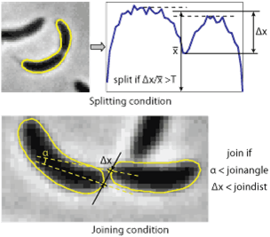
Splitting cells is regulated by splitThreshold parameter. This parameter defines the minimum septation depth in the profile of integrated phase contrast intensity (see the image to the right) which triggers cells splitting. If the condition is met, the program will try to fit new contours to each of the parts of the cells separated by the septum position. Note, if you split the cell manually, this condition does not have to be met. Typical values of the parameter ~ 0.43. The value 1 means that the cell will never be split. If the cells do not split when they should - reduce splitThreshold (to 0.12-0.25), if they split too early - increase it (to 0.4-0.5). In Oufti when a cell divides, both daughter cells get a unique identification number. For example, if there are 100 cells in a given frame and cell # 100 divides, the two daughter cells will be 101 and 102.
Joining cells. The program will attempt to join two cells if the distance between two poles is below joindist parameter and the angle between the axes of the cells at those poles is below joinangle parameter (in radians). If these conditions are met the program will try to fit a new shape to the two cells and check the splitting condition for the resulting cell. Only in this condition fails, the new cell outline will be kept. Note, if you join the cells manually no check for either of the conditions will be performed, however the program needs to be able to fit new shape to the both cells. Typical values are 5 pixels for the distance and ~ 1 radian for the angle, the values can be easily estimated by looking at a highly zoomed image.

Alignment

Parameter Testing.

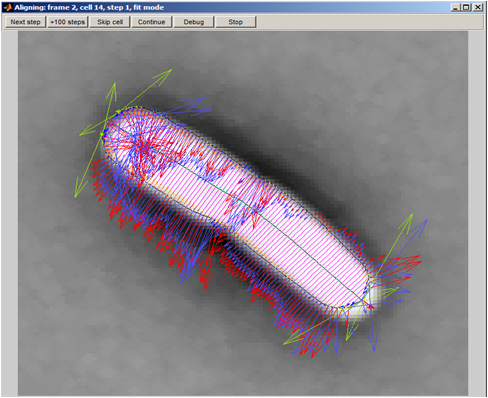
The Alignment button on the Parameter testing panel panel lets the user see the process of alignment dynamically. This module only works with algorithm subpixel. After activating this mode, select a cell, activate the Selected cells only by clicking the box and click on This frame button. This module can also be activated by setting the fitDisplay parameter value to 1. The default value is 0.

Buttons of the alignment tool

Next step - proceed one step and display the new outline
+100 steps - perform 99 steps silently and display the outline of the 100's one
Skip cell - finish the alignment of this cell silently
Continue - finish the alignment of this cell displaying every step without the need to press any button again
Debug - stop Oufti in debug mode (for example, to see the actual values of the forces)
Stop - terminate the process and exits Oufti

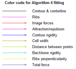
The color codes are used to display the outline and forces for algorithm subpixel and are shown on the second figure.

Fluorescence profiles

To learn how fluorescent profiles are computed, follow the tutorial shown here .

spotDetection

The spotDetection module detects round fluorescent spots inside bacterial cells outlined with Oufti and places them into the meshes structure produced by Oufti.

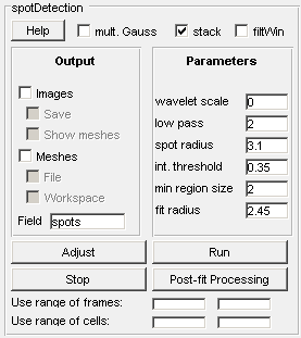
One can use cell mesh data acquired in the cell detection mode with addition of signal channels (see) to quantify spots. Once a user clicks on the spotDetection button on a GUI panel, a spotDetection panel is created in place of the Detection and Analysis panel as shown below.

Output

Images - displays images with detected cells

Save - saves the images (the name of the first image will be requested and subsequent names will be incremented)
Show meshes - displays meshes when displaying images

Meshes - save meshes

File - output them to a file (the program will ask for the file name - .mat format is the default format).
Workspace - When analysis is done from within MATLAB, result data is saved to the workspace.

Other controls

Help - displays this page in a MATLAB browser;
mult. Gauss - The default mode is single 2-D Gaussian model, however, if a user decides to use mixture of 2D gaussians for fitting this box needs to be checked.
Use stack files - loads images from stack files (multiple single channel formats are supported);
filtWin - displays the result of filtering. This is useful for users to pick correct values for filter parameters.
Adjust - run adjustment mode to get the right parameters by clicking on the Adjust button.
Run - run the analysis for every cell in the data set.
The range of frames to use for parameter adjustment and spotDetection; empty fields correspond to the beginning / end of the whole range.

Adjustment mode controls

Previous/Next or left/right arrow on the keyboard - go to the previous/next cell to validate the parameters being used.
Stop - terminate the adjustment mode; the parameters are updated automatically
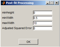
Post-fit Processing - A new window (shown to the right) appears to show post-processing parameters that can be adjusted. The parameters are saved after pressing the OK button. To check the newly changed parameters either press Next or Previous to see their effect on spot analysis.

Parameters

There are two sets of parameters; the first set is shown in the main window of spotDetection under Parameters panel while the second set is triggered by pressing on the Post-fit Processing button.

spotDetection uses a mixture of spatial filtering to acquire regions of interest. These regions of interest are then passed to a 2-D Gaussian or a mixture of Gaussian module for further processing. To analyze crowded and occluded regions both wavelet and band-pass filtering are typically used (typical parameters are; scale -> 1, low pass -> 2, min region size -> 1, spot radius -> 3.1, int. threshold -> 0.2, and fit radius -> 2).

To analyze well seperated spots or single spots, one could only use the band-pass filtering by setting the scale value to be 0.

To analyze beads acquired at different z-stacks one could start of with these parameters (scale -> 2, low pass -> 4, min region size -> 10, spot radius -> 3.5, int. threshold -> 0.2, fit radius -> 6).

To accurately test the Pre-Gaussian fit Parameters, enable the filtWin box (located at the top of the panel). This outputs the result of spatial filtering as regions of interest in a figure mode. These regions of interest are then passed to the mixture of Gaussian module for further processing.

Pre-Gaussian fit Parameters

wavelet scale - The number of image decompositions applied in wavelet analysis. The default value of 2 works in most cases. To not perform wavelet filtering, set this value to 0. Note, when the scale value is set to 0, low pass parameter becomes irrelevant.
low pass - A value of 2 is useful for crowded regions. Larger values makes the feature more smoothed or blurred, thus removing high frequency components between pixel values.
spot radius - Integer length in pixels, 1 or 2 pixels higher than the spots being analyzed. This value is used for high-pass filter, thus removing background noise and helping in feature enhancement.
int. threshold - Applied as a threshold for the amplitude of the signal usefull in removing background noise. The value to be chosen is between 0 and 1.
min region size - Minimum number of pixels a spot must have in order to attempt fitting. For example, the result acquired right after spatial filtering could have a blob or region of interest that is 4 pixels. To drop this region from further processing, set the value of min region size to 5.
fit radius - The amount of distance from peak location. The pixel values inside the circular region are then passed to 2-D Gaussian fitting.

Post-Gaussian fit Parameters

minHeight - minimum height or amplitude of spots to be allowed in image units.
minWidth - minimum width of spots in pixel units.
maxWidth - maximum width of spots in pixel units.
Adjusted Squared Error - minimum threshold for adjusted squared error to be used as a measure for good fit.

Output format

The output format is based on that of Oufti. If output of Oufti was saved as a .txt file then it first needs to be loaded into Oufti by enabling the High-throughput box in the top-panel

The output is saved as a structure with numerous fields as listed below to each cell of the Oufti's cellList.

l - coordinate along the centerline.
d - signed distance from the centerline.
x - euclidian coordinate from the left of the image.
y - euclidian coordinate from the top of the image.
position - segment number in which the spot is located. The spot can be outside of the cell if nonzero Expand cell parameter is used, in which case position would be zero.
adj. Rsquared - The goodness of fit. The value is between 0 and 1, where 1 indicates almost perfect fit.
confidenceInterval_x_y - The 95 percent confidence bounds of the parameters x and y of the fit. The x and y are the coordinate values of the spot.

Before running spotDetection, take a glimpse on how the module works by going here.

objectDetection

The objectDetection module identifies image objects which are larger than the diffraction limit and does so with sub-pixel resolution. Unlike localization of diffraction-limited spots, which have a precise signal expectation, objectDetection identifies the boundaries from the convolution of many points located within the diffraction limit of one another. As a result, the boundaries of the detected objects have less precision than those from the detection of diffraction limited spots.When objectDetection is run, background subtraction is performed first and then a Laplacian of Gaussian kernel is implemented to identify image edges on an up-sampled image. Each of these steps has its own parameters that are exposed to the user.

To run objectDetection, first compute meshes for all the frames or images. See for more information on this. Once the cellList containing all the meshes are computed or loaded into Oufti then load the signal of interest by pressing on Load signal 1 button. This process should be repeated if more than one signal type is being analyzed.

Note: Each analyzed result should be saved to distinct output if more than one signal type is being detected.

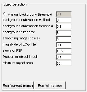
Parameters

Manual background selection - The radiobutton must be activated first, the image will threshold at the level determined by the user. The default value of 0.1 can be changed to any specified value.
Background subtraction method - several options for background subtraction are available, each have varying performance depending on the signal.

1: Subtracts the mean of pixels within the cell
2: Subtracts the noise level determined from objects that are less than or equal to the diffraction limit in size
3: Performs method 1 and then method 2 sequentially.
4: Implements Otsu's method on pixels located within cell outlines to determine which pixels are noise and which are signal. Tends to work very well with DAPI images.

Background subtraction threshold - Used for background subtraction method 2 only. The value specified will be used for determining pixels that are noise or signal.
Background filter size - the number of pixels corresponding to approximately the average diameter of the feature(s) to be extracted. Objects detected of this size or greater are assumed to be signal and not noise. Image noise is determined from the inverse of this filter.
Smoothing range (pixels) - an approximate contour in pixels of the smallest feature to be detected. Larger values will average the outline over a larger image region and produce a smoother outline. Decreasing this value will produce more rigid outlines that will follow image contours more closely. Values smaller than 2 tend to be very sensitive to image noise.
Magnitude of the LOG filter - determines how selective objectDetection will be Larger values will demand that objects to be included have greater contrast to background pixels. Conversely, small values will be more permissive of object edges.
Sigma of PSF - sigma of the point spread function on your optical set-up when it is approximated by a 2-D Gaussian function.
Fraction of object in cell - the minimum fraction of the object to be located within cell boundaries for detection.
Minimum object area - minimum area (in pixels) of detected objects. Objects smaller than this limit will be discarded.

Output

The outlines of detected objects are returned as fields in the cellist for the corresponding biological cell in a given frame. The output for each biological cell is a cell array of n by 2 vectors (corresponding to image X and Y coordinates) specifying the vertices of detected objects.

To run objectDetection, please follow the tutorial objectDetection

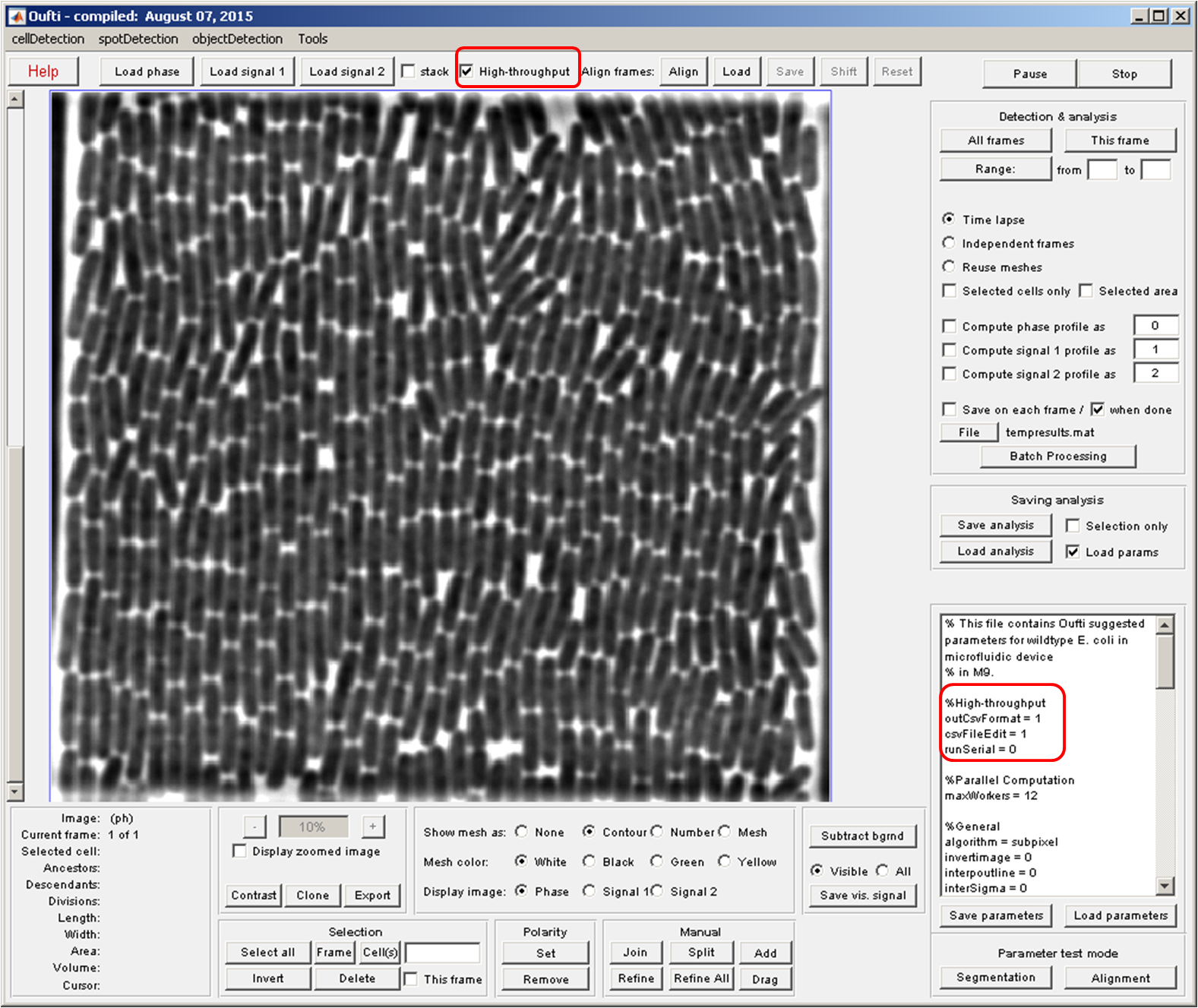
High-throughput

Large image data-sets with very crowded field of view can be processed with Oufti. The following tutorial can be used for any such study besides a microfluidic time-lapse experiment.

Saving Data

.mat

To save the data in .mat format, leave the default value of parameter outCsvFormat as is which is 0.
Click on the High-throughput box to activate analysis for large data sets.
The rest of the analysis is similar to how one would proceed withTime lapse analysis.

.out

For .out format both outCsvFormat and High-throughput box need to be activated, i.e., outCsvFormat = 1 and High-throughput box clicked.
Choose the name of the filename where data needs to be saved such as "test1" by clicking on the File button. This will prompt Matlab to open a writeable file on the specified directory where data will be saved after each processed frame.
Now process the first frame very carefully to only leave out cells that are going to be processed in subsequent frames.
Once the cells are ready to be processed, click All frames or desired range to process the rest of the frames.

Editing Frames

The process to edit a frame by adding, deleting, or modifying cells is different in the .out format. To edit frames remember the following:

The csvFileEdit parameter should be set to 1 in the parameter window.
Once a particular frame is edited, all frames following must be reprocessed to update the changes you made.

Loading data

.mat

To load the data in .mat format, the outCsvFormat parameter should be set to 0 (this is the default).
Click on the High-throughput box to activate saving data in .out format.
Click on the Load analysis button and select the .mat file if you want to load.

.out

To load data in .out format, the outCsvFormat parameter should be set to 1 and the High-throughput box should be selected.
Click on Load analysis button and select the file (.out) to load.

Top

Tutorial