
Data Visualization and Evaluation
cellCycleViewer
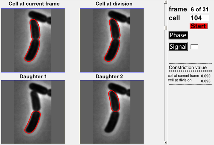
This module is designed to help users visualize a division cycle for a particular cell in a time-lapse experiment. The default mode for the image is phase-contrast but one can also display fluorescent signals by specifying the identifier for the fluorescent signal and activating the ‘Signal’ toggle button. A scrollbar is also provided so that users can scroll between the different frames in the cell cycle to view constriction value (also calculated and shown in the module) and cell outlines.
The module works with image and cellList data. The image data can be loaded into the Oufti application while the cellList data is gathered through the analysis of images.
Procedures
- Select the number of cell for which to view the cell cycle.
- Click on either Phase button or Signal button. For Signal button make sure to enter a value such as 1 or 2.
- Click the Start button to generate the full cell cycle for the selected cell. Note; if a cell cycle is not detected, nothing will be shown.
spotViewer
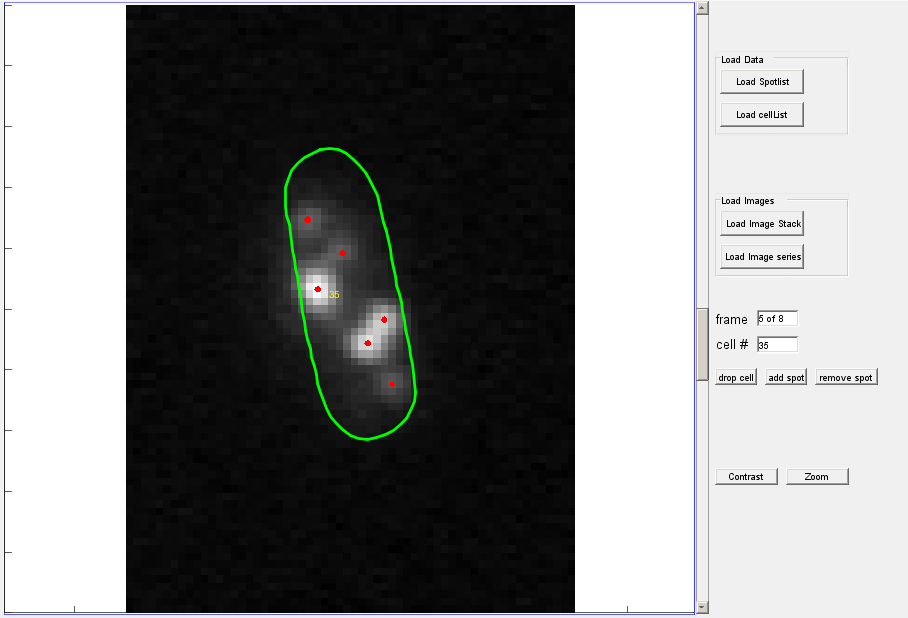
The spotViewer module is designed to aid in visualization and evaluation of data collected after analysis is completed in the spotDetection module. This application enables one to manually add a spot or remove a false-positive spot that was gathered in the spotDetection module. The module provides a ‘zoom’ and ‘contrast’ options to help visualize spots.
To use the spot addition or deletion option, enter the cell number in which the spot is located, into specified box. The utility also provides an option to remove the whole cell structure from the analysis by pressing the drop cell button.
Procedures
- Load the cellList.
- Load the signal images.
movieConstruction
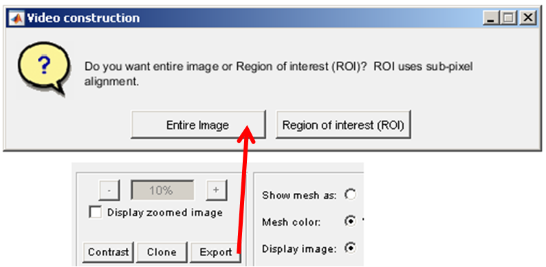
The movie construction module can produce movies from frames/images with Oufti processed outlines (by pressing the Entire button) or can construct videos for regions of interest with sub-pixel resolution (by selecting the ROI button).
Entire image
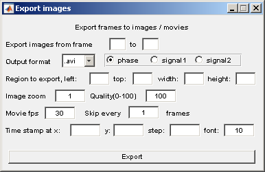 The parameters for this sub-module are self explainatory. The unit for the location parameters, e.g; Region to export is pixels.
Region of interest (ROI)
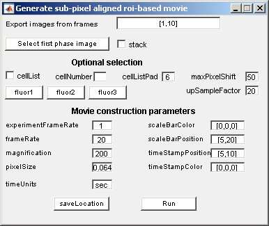
Procedures
- Choose the frame range.
- Load the phase images by clicking the Select first phase image button.
- Load the corresponding fluorescent images by clicking on Fluor1, Fluor2, etc.
- If the cellList box is selected, also select the cellNumber for region of interest.
- To specify a region of interest un-check the cellList box.
Cell dimensions statistics
cell statistics
Applying this function to the already processed data provides one with statistics (total number of cells, cell length, cell width, cell area, and cell volume) for the whole cell population. This function also provides information (total number of spots, total signal intensity, and signal intensity normalized by area) on the spots structure if present in cellList structure data.
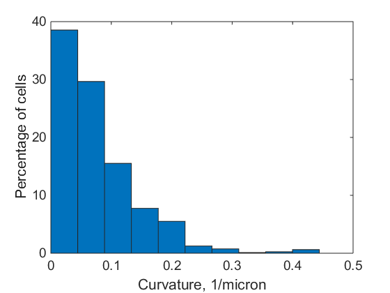
curvature histogram
This function plots a histogram of the curvature of all the cells analyzed by Oufti.
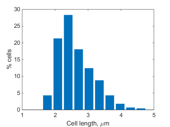
length histogram
This function plots a histogram of the length of all the cells in a population.
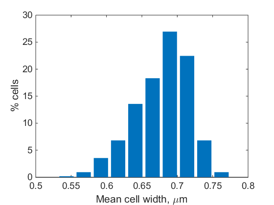
mean width histogram
This function plots a histogram of the mean width of every cell in a population
Cell intensity statistics
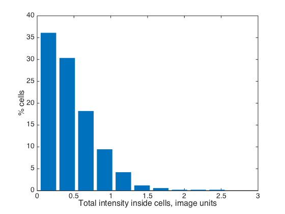
signal intensity histogram
This function plots a histogram of the total intensity inside every cell in a population. Note, the background has to be subtracted before detecting the signal in Oufti. The GUI provides users the ability to subtract background from every signal image. This is done by first loading the phase images, followed by signal images.
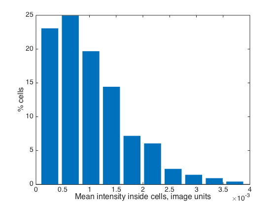
mean intensity histogram
This function plots a histogram of the mean intensity inside every cell in a population, i.e. total intensity divided by the area of the cell. Note, the background has to be subtracted before detecting the signal in Oufti. The GUI provides users the ability to subtract background from every signal image. This is done by first loading the phase images, followed by signal images.
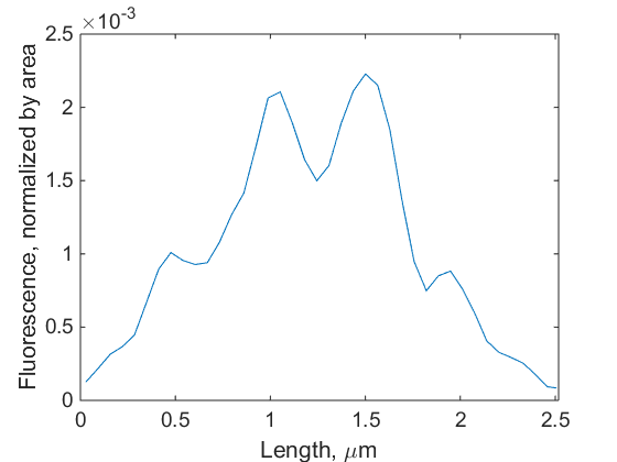
intensity profile
This function plots the intensity profile for a single cell. Note, the background has to be subtracted before detecting the signal in Oufti. The GUI provides users the ability to subtract background from every signal image. This is done by first loading the phase images, followed by signal images.
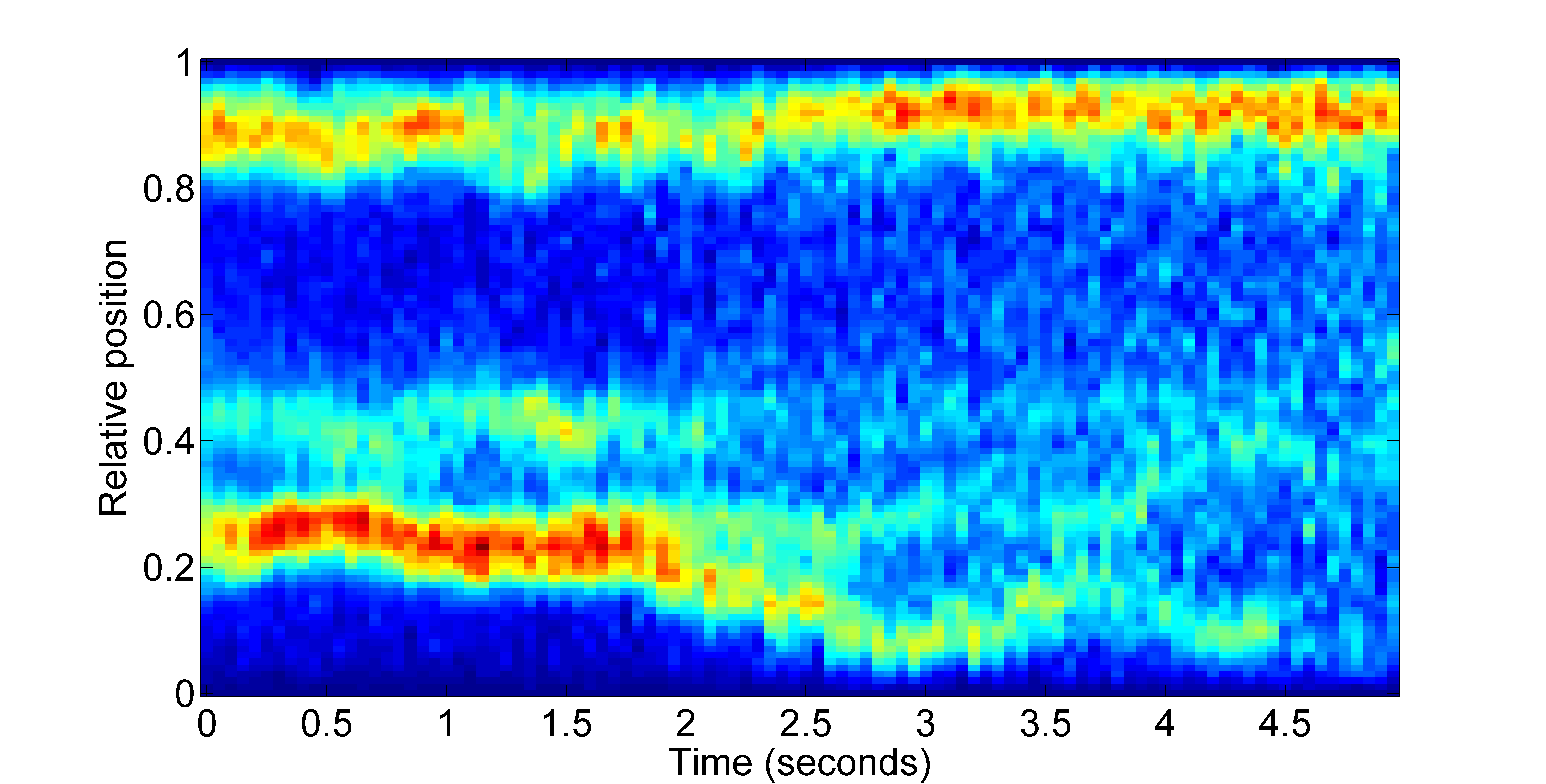
kymograph
The kymograph function produces an intensity heatmap for any signal value in a time-series fashion. In Oufti, the signal profile can be obtained as shown here. Once the signal profile for the different fluorescent signals inside the cells are obtained, the kymograph module can be used to visualize the intensity map of the fluorescent profile over time. The intensity map is created by first computing the interpolation of the original data in fifty equidistant points spanning the interval 0 to 1. This linear interpolation is followed by integration in the interval 0 to 1. This operation is performed on each specified time point and the final result is presented as a kymograph.
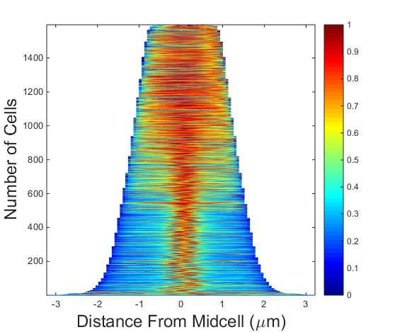
demograph
This function generates a demograph of the signal profile for a single cell through a time series obtained by Oufti. Demographs are constructed by first integrating the signal values in each segment of the cell mesh and then normalizing the fluorescence in each cell by the maximum integrated value of a particular segment. After this, cells are sorted by the cell length value and the fluorescence values are plotted as a heat map, where 0 corresponds to 0 and 1 to maximum fluorescence signal in the segment of the cell mesh.
Displaying cells and spots
display cell
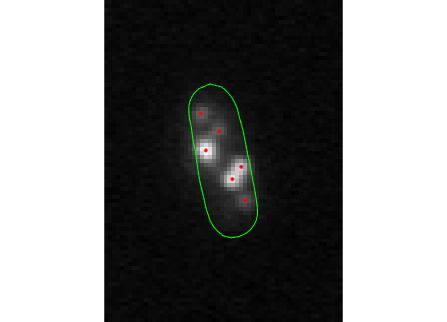
This function displays a selected cell, including the contour and all identified spots.
display all cells
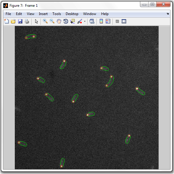
This function displays a full frame including all the detected cells and identified spots (if present).
Growth curves and cellList filtering
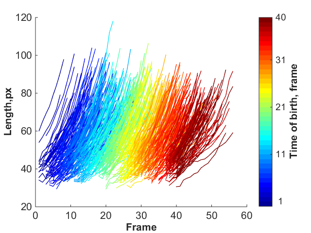
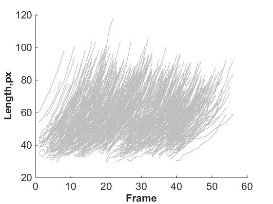
growth curves
With this function, users can view the growth curves of individual cells over their entire cell cycle. The
function assumes that the cell detection part of the analysis is done prior to using this tool.
Assuming the cell detection part is done, users can get a plot similar to the one shown by selecting the Tools tab in the GUI and then pressing on the selection
growth curves.
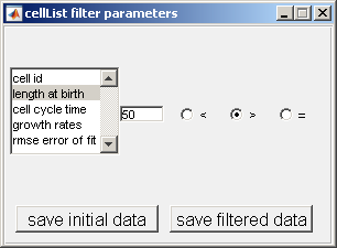
cellListFilter
This module allows the user to view subsets of a given population, by filtering cells using parameters shown in the cellListFilter parameters window.
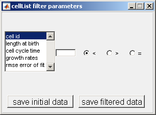
For example, one could desire to
see all cells with a length at birth greater than 50 pixels. To filter based on length at birth from the selection window, insert '50' in the box and
select the button > as shown below.
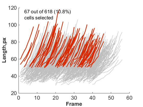
Once one of the markers for a given parameter is selected, a plot will be created. This plot will show red lines to represent data points selected through the
filtering process, and grey lines to represent all omitted points. This filtered data, as well as original un-filtered data can be saved using the buttons
provided in the cellListFilter parameters window.
The fields in the structure returned by the save filtered data button are:
- id: Vector of ID numbers of the cells tracked over time.
- Lbirth: Vector of length at birth. The order of the Lbirth Vector matches the order of the Vector of cell id numbers (field ‘id’).
- Length: cell array of vectors recording the cell length of each cell along their life cycle. Each entry of the cell array represents one cell as one vector of
length as long as the number of frames in which this cell was detected. The order of the cell array entries matches the order of the array of cell id numbers (field ‘id’).
- Frame: Same as the field ‘length’ but with the frame number at which the cell was detected. The vectors of frame numbers correspond to the vectors of cell length.
- Cct: Vector of inter-division times, in frames, calculated as the time elapsed between the detected birth and the detected division.
- gRate: Vector of relative growth rates (frame-1) calculated by fitting a linear model to the relation log(length)=f(time).
The fitting step is made robust by excluding the data points that lay more than 2 standard deviations away from the mean of the residuals.
- rmseFit: Vector of the root mean squared errors of the fit applied to calculate the growth rate based on the growth curve.
- Rmsd: Vector of the root mean squared deviations of the logarithm of the ratios of two lengths measured consecutively.
For each cell the vector of cell lengths is normalized by the length at birth (Li/L0).
The logarithm of this normalized vector is differentiated (diff(log(Li/L0)) and the r.m.s.d. for this vector is computed and returned into the field ‘rmsd’.
Export and Import cellList data
export cellList to text-format data
This module converts the cellList format to a ".csv" format. The ".csv" format is a comma-delimited format that can be analyzed in Excel.
The structure of the ".csv" format is;
- Title: The name and path of the file as well as the date of creation.
The parameters used for the cell contour detection are listed at the beginning of the file. Each parameter is reported on a new line starting with #.
- $shiftframe: Reports the frame shifts, in pixels, from one image to the next, if computed prior to the analysis.
- $cellListN: Reports the number of cells detected per frame.
- %parameter values: Reports the values of each parameter for all cells in all frames. Each line (starting with #) refers to one detected cell;
each parameter value is separated with a comma. In the case of a parameter represented by an array of values, these values appear separated by spaces.
For an array that has more than one column, the different columns are separated by semicolon (;).
- Fame Number: Frame number in which the cell is detected
- Ancestors: Cell ID number of the mother cell, if any.
- Birthframe: Most useful in time lapses, this parameter records the frame number at which the cell was first detected.
- Box: An array of 4 values, in pixels, defining the bounding box of the cell. Use this values to crop the image and display this specific cell. The box parameter values are the same as in the *.mat format ([bottom, left, width, height]);
- Descendants: Cell ID number(s) of the detected descendants of this cell.
- Divisions: Frame at which a cell divides. This parameter value is useful in time lapse experiments and is filled in at the last frame at which a cell, as defined by its ID number, is detected.
- Mesh: An array of four columns, in pixels, specifying the location of the cell edges in image coordinates. As for the *.mat version, the mesh parameter (or field) is organized in 4 series of numbers (x1 y1 x2 y2). Series of numbers are separated by “;” while numbers within a series are space-separated. The vectors x1, y1 define one side of the cell while x2, y2 define the other side. Both half contours start and end at the same points ([x1(1),y1(1)] = [x2(1),y2(1)]).
- Length: Cell length in pixels
- Area: Cell area in pixels
- Polarity: Value defining the polarity of the cell.
- Signal0: Array of values, in arbitrary units, specifying the intensity profile along the cell length. The length of the vector has the same length as the cell mesh (x1, y1, x2 or y2) and each values corresponds to a cell segment defined by the cell mesh.
- spots: [a1 a2 an; b1 b2 bn; ...], where numericals refer to the number of spots in a given cell and the alphabets refer to the sub-fields. The sub-fields are in this order; l, d, x, y, positions, and adj. Rsquared. See for more information.
- objects: [a1 a2 an; b1 b2 bn; ...], where numericals refer to the number of objects in a given cell and the alphabets refer to the sub-fields. The sub-fields are in this order; outlines, pixels, pixelvals, and area. The outlines sub-field is a 2-by-n array of sub-pixel location values. The first column refers to the x-locations while the second columns refers to y-locations, pixels are image unit values indicating location of nuleoids in image coordinates, pixelvals are the pixel values of each pixel location shown in pixels sub-field, and area sub-field is the calculated area of each nucleoid.
When spotDetection or objectDetection is used, extra fields of spots or objects are created in the cellList. The program will automatically check for the presence of these extra fields. If present, these fields will be exported to a comma-dilimited text file with headings spots or objects. However, the sub-fields are structured as semicolon dilimited as shown below;
import text-format data to cellList
Text-format data generated through the High-throughput mode can be converted back to Matlab format. This is useful for those who want to perform post-processing on already processed image datasets in Matlab. Note: Make sure that, 'global cellList' is called in the Matlab command window.
In some circumstances when the ".out" file is large and does not need to be converted to cellList, the users have the option to go through the large data set and import chunks of data in to Matlab. There are different ways to do this and one suggestion would be to use the following command lines.